Problems with spaces and text

11/6/2020

Remove spaces that cause #VALUE!

Often #VALUE! occurs because your formula refers to other cells that contain spaces, or even trickier: hidden spaces. These spaces can make a cell look blank, when in fact they are not blank.

1. Select referenced cells

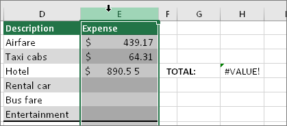
Find cells that your formula is referencing and select them. In many cases removing spaces for an entire column is a good practice because you can replace more than one space at a time. In this example, clicking the E selects the entire column.

2. Find and replace

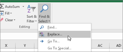
On the Home tab, click Find & Select > Replace.

3. Replace spaces with nothing

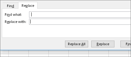
In the Find what box, type a single space. Then, in the Replace with box, delete anything that might be there.

4. Replace or Replace all

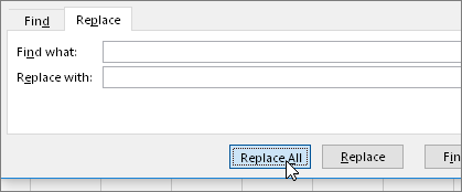
If you are confident that all spaces in the column should be removed, click Replace All. If you'd like to step through and replace spaces with nothing on an individual basis, you can click Find next first, and then click Replace when you are confident the space isn't needed. When you're done, the #VALUE! error may be resolved. If not, go to the next step.

5. Turn on the filter

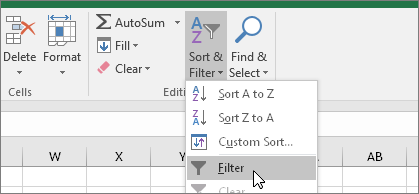
Sometimes there are hidden characters other than spaces that can make a cell appear blank, when it's not really blank. Single apostrophes within a cell can do this. To get rid of these characters in a column, turn on the filter by going to Home > Sort & Filter > Filter.

6. Set the filter

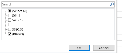
Click the filter arrow  , and then deselect Select all. Then, select the Blanks checkbox.

7. Select any unnamed checkboxes

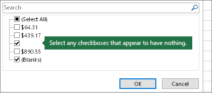
Select any check boxes that don't have anything next to them, like this one.

8. Select blank cells, and delete

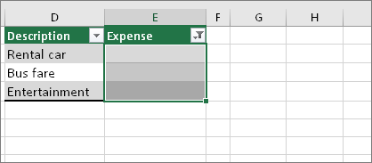
When Excel brings back the blank cells, select them. Then press the Delete key. This will clear any hidden characters in the cells.

9. Clear the filter

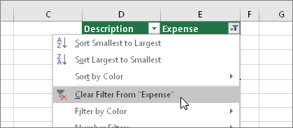
Click the filter arrow  , and then click Clear filter from... so that all cells are visible.

10. Result

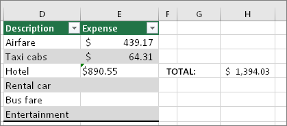
If spaces were the culprit of your #VALUE! error then hopefully your error has been replaced by the formula result, as shown here in our example. If not, repeat this process for other cells that your formula refers to. Or, try other solutions on this page.

Note: In this example, notice that cell E4 has a green triangle and the number is aligned to the left. This means the number is stored as text. This may cause more problems later. If you see this problem, we recommend converting numbers stored as text to numbers.

Example with #VALUE!

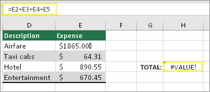
Here’s an example of a formula that has a #VALUE! error. This is likely due to cell E2. There is a special character that appears as a small box after "00." Or as the next picture shows, you could use the ISTEXT function in a separate column to check for text.

Same example, with ISTEXT

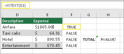
Here the ISTEXT function was added in column F. All cells are fine except the one with the value of TRUE. This means cell E2 has text. To resolve this, you could delete the cell's contents and retype the value of 1865.00. Or you could also use the CLEAN function to clean out characters, or use the REPLACE function to replace special characters with other values.

After using CLEAN or REPLACE, you'll want to copy the result, and use Home > Paste > Paste Special > Values. You might also have to convert numbers stored as text to numbers.

Source: Support.microsoft.com