Problems with subtraction

11/6/2020

How to do basic subtraction

If you're new to Excel, you might be typing a formula for subtraction incorrectly. Here are two ways to do it:

Subtract a cell reference from another

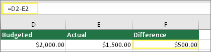
Type two values in two separate cells. In a third cell, subtract one cell reference from the other. In this example, cell D2 has the budgeted amount, and cell E2 has the actual amount. F2 has the formula =D2-E2.

Or, use SUM with positive and negative numbers

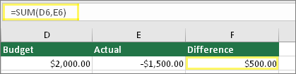
Type a positive value in one cell, and a negative value in another. In a third cell, use the SUM function to add the two cells together. In this example, cell D6 has the budgeted amount, and cell E6 has the actual amount as a negative number. F6 has the formula =SUM(D6,E6).

1. First do a quick test. In a new workbook, type a 2 in cell A1. Type a 4 in cell B1. Then in C1 type this formula =B1-A1. If you get the #VALUE! error, go to the next step. If you don't get the error, try other solutions on this page.
2. In Windows, open your Region control panel.
   • Windows 10: Click Start, type Region, and then click the Region control panel.
   • Windows 8: At the Start screen, type Region, click Settings, and then click Region.
   • Windows 7: Click Start and then type Region, and then click Region and language.
3. On the Formats tab, click Additional settings.
4. Look for the List separator. If the List separator is set to the minus sign, change it to something else. For example, a comma is a common list separator. The semicolon is also common. However, another list separator might be more appropriate for your particular region.
5. Click OK.
6. Open your workbook. If a cell contains a #VALUE! error, double-click to edit it.
7. If there are commas where there should be minus signs for subtraction, change them to minus signs.
8. Press ENTER.

Repeat this process for other cells that have the error.

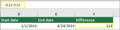
Type two dates in two separate cells. In a third cell, subtract one cell reference from the other. In this example, cell D10 has the start date, and cell E10 has the End date. F10 has the formula =E10-D10.

Or, use the DATEDIF function

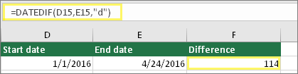
Type two dates in two separate cells. In a third cell, use the DATEDIF function to find the difference in dates. For more information on the DATEDIF function, see Calculate the difference between two dates.

Check for leading spaces

1. Double-click a date that is being used in a subtraction formula.
2. Put your cursor at the beginning and see if you can select one or more spaces. Here's what a selected space looks like at the beginning of a cell: 

If your cell has this problem, proceed to the next step. If you don't see one or more spaces, go to the next section on checking your computer's date settings.

3. Select the column that contains the date by clicking its column header.
4. Click Data > Text to Columns.
5. Click Next twice.
6. On Step 3 of 3 of the wizard, under Column data format, click Date.
7. Choose a date format, and then click Finish.
8. Repeat this process for other columns to ensure they don't contain leading spaces before dates.

Check your computer's date settings

Excel uses your computer's date system. If a cell's date isn't entered using the same date system, then Excel won't recognize it as a true date.

For example, let's say that your computer displays dates as mm/dd/yyyy. If you typed a date like that in a cell, Excel would recognize it as a date and you'd be able to use it in a subtraction formula. However, if you typed a date like dd/mm/yy, then Excel wouldn't recognize that as a date. Instead, it would treat it as text.

There are two solutions to this problem: You could change the date system that your computer uses to match the date system you want to type in Excel. Or, in Excel you could create a new column and use the DATE function to create a true date based on the date stored as text. Here's how to do that assuming your computers date system is mm/dd/yyy and your text date is 31/12/2017 in cell A1:

1. Create a formula like this: =DATE(RIGHT(A1,4),MID(A1,4,2),LEFT(A1,2))
2. The result would be 12/31/2017.
3. If you want the format to appear like dd/mm/yy, press CTRL+1 (or  + 1 on the Mac).
4. Choose a different locale that uses the dd/mm/yy format, for example, English (United Kingdom). When you're done applying the format, the result would be 31/12/2017 and it would be a true date, not a text date.

Note: The formula above is written with the DATE, RIGHT, MID, and LEFT functions. Please notice that it is written with an assumption that the text date has two characters for days, two characters for months, and four characters for year. You may need to customize the formula to suit your date.

Source: Support.microsoft.com